Archive for March, 2009

Stat 295, 3/26/09

March 27, 2009

Please note: The homework for next week has been posted in the immediately preceding blog entry. It is due on Thursday.

Comments on the homework: Some groups have been having difficulty writing down the likelihood. The likelihood for observation j is \lambda^{y_j} \exp(-\lambda)/y_j! Some were writing the first term over all data as \lambda^{\vec{y}}. What does that mean? There is no such thing. They should have written \lambda^{\sum{y_j}}, which is the product of the individual likelihoods for each observation, so that the likelihood to use should have been \lambda^{\sum{y_j}}\exp(-n\lambda), where n is the number of observations.

Other problem: People were programming the Gibbs sampler…They were not updating the value of the variables sent to sample1(). Need betas[i]=beta=z$beta; that middle assignment is critical. Without it, you are always sending the same position to the sampler, and it won’t move around as it should.

There was a perfect paper by undergrads in the course; the grad students need to match this!

We were talking about the linear regression model from last time, which was, you recall:

y_i=\beta_0+\beta_1 x_{1j}+\beta_2 x_{2j}

So we looked at the plots. We fit the least squares model using R function lm(), which gives the frequentist result. We looked at confidence intervals and point estimates.

For our Bayesian analysis we’ll put independent priors as per the blog last time. They were very broad priors that are almost flat. Jeff has learned that it is possible to put flat priors on the betas (but BUGS didn’t let you do that before so that’s why the priors we talked about on Tuesday are proper).

We analyzed the R code and the WinBUGS code.

Then we ran it from R (consult the R code). We looked at the output of the bugs() function in the arm package, which we called linreg.sim (see R code for this); We want Rhat close to 1 to verify good mixing. We looked at the traces, which looked good.

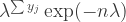
You can define a function and have BUGS evaluate that function over the chain and return a sample. So for example, the usual Rsquare is given by
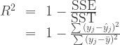
\begin{array}{rclr} R^2 & = & 1-\frac{\mbox{SSE}}{\mbox{SST}} \\ & = & 1-\frac{\sum{(y_j-\hat{y}_j)^2}}{\sum{(y_j-\bar{y})^2}}\end{array}

Adjusted R^2: Divide the fraction’s numerator by (n-p) and its denominator by (n-1)

In the Bayesian case define

R_B^2=1-\frac{\sigma^2}{s_y^2} where s_y^2 = \frac{1}{n-1}\sum{(y_j-\bar{y})^2}

(closest to the adjusted R^2).

This is in the R code sent to WinBUGS.

typical.y (see the WinBUGS file) computes a posterior distribution on the estimated mean time it takes to service, using mean(cases[]), mean(distance[]).

We talked about other possibly useful features, like the log file, tracing, and the listserv.

Jeff remarked that the best way to learn BUGS is to look at the models that they have as examples.

Next example:

ANOVA models. One-way ANOVA is a useful linear model.

Our example: Interested in whether different exercise programs affect time to walking in infants.

Four different programs, called Active, Passive, No Exercise, Control Group.

Six infants in each group (randomized). Outcome is time in months when infants first walk.

Model:

\begin{array}{rcl}y_{ij}&=&\alpha_i+\epsilon_{ij}\\ \alpha_i & \sim & N(\mu_{\alpha}, \sigma_{\alpha})\\ \epsilon_{ij} & \sim & N(0,\sigma) \end{array}

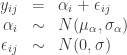
This is a random effects model and also a hierarchical model.

i=\mbox{group}, j=\mbox{infant} within the group.

\alpha_i denotes the mean time to walking in group i. Without the second of these three lines it’s a one-way fixed effects ANOVA model. With it it is a random effects ANOVA model. It’s natural for a Bayesian to put a distribution on \alpha_i so it’s natural (and simple) for her to consider a random effects model.

Assignment #8, Due 4/2/09

March 27, 2009

Here is the pdf file for the eighth problem set, due 4/2/09.

Stat 295, 3/24/09

March 25, 2009

We started with a few words from Bill, who remarked that the idea of Gibbs sampling includes the idea of sampling in turn from various conditional distributions, so that each (vector) parameter \theta_j sampled conditional on the current values of all the other parameters \theta_{-j}, where the dash indicates that \theta_j is omitted. When we did this, we assumed that we could actually sample easily and exactly from the conditional distributions. However, this is usually not possible, and the way around it is to use Metropolis-Hastings sampling on those parameters. This is called “Metropolis-within-Gibbs.”

I remarked that you have to be careful when using Metropolis-Hastings on a parameter (like \sigma^2) that is strictly positive. One way to do this is just to define the posterior conditional distribution on this parameter as zero for \sigma^2\leq 0 so that any attempt to propose in that region will be rejected; a simpler and probably better method is to log-transform the variable: \theta=\log(\sigma^2), for example. This has many advantages. One is that the Jeffreys prior on \sigma^2 is singular at 0, whereas the corresponding prior on \log(\sigma^2) is flat.

Jeff took over to discuss linear models. He remarked that linear models like regression, multiple regression, ANOVA,… are still a huge part of the statistican’s toolkit, even though modern computational power enables us to solve models that previously would have been intractable.

Jeff started with simplest case: Normal, one variable. The problem is estimation from a normal, mean \mu, variance \sigma^2 population. The data are n iid random variables y_1,y_2,...y_n, each N(\mu,\sigma^2). The objective is to estimate (\mu,\sigma).

The likelihood is

f_n(y|\mu,\sigma^2)=(2\pi\sigma^2)^{-n/2} \exp[-S_{yy}/2\sigma^2]exp[-n(\mu-\bar{y})/2\sigma^2],

where \bar{y} is the sample mean and S_{yy}=\sum{(y_j-\bar{y})^2} (you’ve seen this notation before).

We have several cases:

1. \sigma^2 known (this never happens, but it is pedagogically interesting).

We have two subcases:

1a) flat prior on \mu
1b) normal prior on \mu

(1a) is the limiting case of (1b) for when the variance \rightarrow\infty. So the only case Jeff discussed under (1) was (1b).

2. \mu, \sigma^2 both unknown.

Again, we have two cases:

2a. Flat prior on \mu, Jeffreys prior g(\sigma^2)\propto 1/\sigma^2 on \sigma^2.
2b. Conjugate priors, i.e.,

\mu \mid \sigma^2 \sim N(\mu_0,\sqrt{\sigma^2/c_0}),
\sigma^2 \sim\mbox{inv-gamma} (\alpha_0,\beta_0)

(2a) is the limiting case of (2b) when \alpha_0=\beta_0=c_0=0. So Jeff only discussed (2b).

So we really only have to look at two cases:

Jeff then stated, but did not prove, the preliminary result that you are to prove and turn in on 3/26/09. We will find this result very useful.

Case 1b:

g(\mu)=(2 \pi \sigma_0^2)^{-1/2}\exp[-\frac{1}{2 \sigma_0^2} (\mu-\mu_0)^2]

\begin{array}{rclr}g(\mu \mid \vec{y}) & \propto & f_n(\vec{y}\mid\mu)g(\mu) \\ & = & (2 \pi \sigma^2)^{n/2}\exp[-\frac{S_{yy}}{2 \sigma^2} \exp(-\frac{n}{2 \sigma^2} (\mu-\bar{y})^2-\frac{1}{2 \sigma_0^2}(\mu-\mu_0)^2] (2 \pi \sigma_0^2)^{-1/2}\end{array}

Now expand and look at the useful theorem, just read off the answer, which is:

\mu\mid\bar{y} \sim N(w \mu_0 +(1-w)\bar{y},\sqrt{(1-w)\sigma^2/n})

where w=\frac{\sigma^2/n}{\sigma^2/n + \sigma_0^2}

As n\rightarrow\infty, w\rightarrow 0, \mu\rightarrow\bar{y}

as \sigma_0\rightarrow\infty, w\rightarrow 0, \mu\rightarrow\bar{y} and the standard deviation \rightarrow \sqrt{\sigma^2/n}

Note that in this limit we recover the frequentist result (known \sigma, flat prior on \mu).

For large n, \mu\mid \vec{y} \sim N(\bar{y},\sigma/\sqrt{n})

Case 2b: \mu,\sigma^2 unknown, \mu \mid \sigma^2 \sim N(\mu_0,\sqrt{\sigma^2/c_0}),

\sigma^2 \sim\mbox{inv-gamma} (\alpha_0,\beta_0)

The calculation for \mu \mid \vec{y},\sigma^2 is very similar to case (1a). See the notes. The result is

\mu\mid\sigma^2,\vec{y} \sim N(w \mu_0 + (1-w)\bar{y},\sqrt{(1-w)\sigma^2/n}),

where w=\frac{\sigma^2/n}{\sigma^2/n + \sigma_0^2}, \sigma_0^2=\sigma^/c_0

\sigma^2 \mid \vec{y} \sim \mbox{inv-gamma} (\alpha_0+(n-1)/2, \beta_0+S_{yy}/2)

Priors and posteriors are in same family, they are conjugate.

Specific example: two predictors.

Linear regression. We’ll start with a specific example and perhaps do some general theory later. The example comes from “Bayesian Modeling Using WinBUGS” by Ntzoufras.

Example: We are interested in understanding the relation between total service time (minutes) of restocking vending machines and two predictors, x_1 is the number of cases stocked, x_2 is the distance in feet from the truck to the machine.

Model: y_i=\beta_0+\beta_1 x_{1i}+\beta_2 x_{2i} + \epsilon_i for i=1,…,25

Assume that the errors are N(0,\sigma^2) and independent (\perp). Let \tau=1/\sigma^2\equiv precision.

We’ll use INDEPENDENT priors on (\beta_0, \beta_1, \beta_2) and \tau, specifically \beta_i \sim N(0,\sqrt{10^4}) and \tau\simgamma(0.01,0.01)

We learned that Control-R or right-click selected region to run it in R (at least for Windows).

Note that there is a WinBUGS listserv discussion list.

A package called “arm” allows you to call WinBUGS via R. Will also need WinBUGS itself. A patch must be installed, and you must run their immortality key.

To be continued…

Short assignment, due 3/26

March 24, 2009

Jeff wants you to prove this short preliminary result, due on Thursday, 3/26:

For a p-dimensional parameter \theta, if its density

g(\theta) \propto \exp\left[-\frac{1}{2}(\theta^T A \theta -2 b^T \theta)\right],

where A is a p \times p matrix and b a p \times 1 vector, then

\theta \sim N(A^{-1}b, A^{-1})

This is a commonly used technique called “completing the square,” in its general matrix form. It is often needed when working with the kernel of normal distributions (as we did later in the lecture today).

Stat 295, 3/19/09

March 20, 2009

We put up a chart with sufficient conditions for a Markov chain to have as its limiting distribution the target distribution we are interested in. Briefly, the chain (1) must be able to access every state from every other state in a finite number of steps, with nonzero probability; (2) must not contain periodic states (that repeat after a given number of steps); (3) must not shrink.

We showed that if the proposal distribution is q(j \mid i) for any two states i,j, then we satisfy the detailed balance condition by choosing M_j^i=q(j|i)\alpha_j^i where

\alpha_j^i=min\left\{1,\frac{q(i \mid j)\phi_j}{q(j \mid i)\phi_i}\right\}

The procedure for drawing a sample from the posterior distribution becomes:

  1. Start at an arbitrary point i in the state space S
  2. Generate a random variable j from the arbitrary but fixed proposal distribution q(j \mid i). This is a proposed move to a new state.
  3. Calculate \alpha_j^i according to the above prescription.
  4. Generate a U(0,1) random variable u.
  5. If u<\alpha_j^i, then accept j as the new state (the chain moves); if not, keep i as the new state (the chain doesn’t move)

Repeat steps 1-5 until a sufficiently large sample is obtained.

We remarked that it is very important not to discard i if the chain doesn’t move. It is still part of the sample, and if you were to discard it, you would not be sampling from the true posterior distribution. It is possible, and indeed happens frequently, that a chain will not move on every try but will remain in the same position. Those “repeats” are still part of the chain and must be kept. Jeff remarked that when he was learning the Metropolis-Hastings method, he wrote a program that discarded these steps, and was puzzled when the results did not agree with what he knew to be the correct answer. It was only when he fixed the program to keep the repeats that the results were as expected.

(Parenthetically, when you are doing SIR, it is also possible, and expected, that some points will be resampled more than once, since you are sampling with replacement. It would be as wrong to discard those repeats as it is to discard repeats when doing Metropolis-Hastings sampling.)

I remarked that when I actually code the calculation, I omit computing the minimum. It’s not necessary, since if the fraction is greater than 1, you’ll always accept, even if you compare u with the fraction.

Jeff and I warned that it is essential to calculate using logs, and in particular, not to calculate the likelihood and then take the log, but rather to calculate the log likelihood directly, using tricks such as the fact that many of the densities in R have a parameter ‘log’ which, if set to be TRUE (T) will directly give you the log of the density. So, ‘y=dnorm(x,mean=a,sd=sigma,log=T)’ gives you the log of the normal density at x. Obviously, then, you will calculate the log of \alpha_j^i by adding and subtracting the logs of the priors and likelihoods, and compare it to the log of u in deciding whether to accept or reject the proposed move.

We ran the simple program in the notes. We found that it’s important with this kind of symmetric proposal (that is, the proposal density is an even function, centered on the current position), that the density not try proposed steps that were too far from the current position (otherwise the sampler will remain for long periods at the same point before it eventually proposes a step that will be accepted, because the sampler would propose a lot of points in the tails of the target distribution, which will probably be rejected since the \alpha_j^i will be very small. Similarly, we found that if the steps proposed were all small because the width of the proposal distribution is to small, then most steps will be accepted, but the sampler will take a long time to get anywhere. Typically, you want the proposal distribution for this kind of sampler to have a width that is comparable to several standard deviations of the posterior distribution.

We found that if we started way off of the peak of the posterior distribution, it may take quite a while before the sampler moves into a region that mixes well. This is why we discard the beginning of the sample…the “burn-in”. We also pointed out that a good technique is to run several different chains, starting at different points, to see if the inferences we get are similar. This is a good sanity check.

Finally, we remarked that the larger the sample, the better the inferences from the sample will be. We noted that we are actually using frequentist ideas when we calculate means, medians, standard deviations, quantiles, etc., from the sample. This may be regarded by some as ironic. We also noted that the precision of the inferences will improve with sample size N proportionally to \sqrt{N}, so there is a point where taking more and more samples doesn’t improve things much. The standard deviation of our estimate of the posterior mean, for example, only improves by a factor of about 3 when we take 10 times as many samples, and 10 if we take 100 times as many samples. I also pointed out that taking more and more points doesn’t change things like the standard deviation of the posterior distribution; but it does improve our estimate of that standard deviation.

Misleading statistics

March 19, 2009

Andrew Gelman has an interesting blog entry today on basketball. It shows how inferences depend on the model and how model error can lead to silly results. (Nothing particularly Bayesian, but a good lesson in statistics).

Stat 295, 3/17/09

March 18, 2009

Is my face red! I apologize to each and every one of you for being late to class today.

Today we introduced the idea of Markov chains. Recall that a stochastic process is a sequence \{X_1,X_2,...,X_n,...\} of random variables on some state space S indexed by a discrete index set (e.g., the integers). A Markov chain is a stochastic process with the property that P(X_{n+1}|X_1,X_2,...,X_n)=P(X_{n+1}|X_n), that is, each each state depends only in the immediately preceding state and is independent of all of the states before that; the Markov chain has no “memory” of exactly how it got to the last state.

A Markov chain is stationary if the transition probabilities are independent of the index, that is, if P(X_{n+1}=j|X_n=k) does not depend on the value of n. A stationary Markov chain is characterized by a transition matrix M_j^k=P(X_{n+1}=j|X_n=k), also known as the Markov matrix. The entries of the Markov matrix satisfy 0\le M_j^k \le 1 and, since every state k must go somewhere, probability must be conserved and \sum_j M_j^k=1.

A stationary distribution of a Markov chain is a distribution \pi over the states such that \pi_j \geq 0 for all j, and \pi = M \pi.

We remarked that we are going to study Markov chains in a somewhat “backwards” way from the way they are usually studied. Usually, we are given the Markov matrix M and asked to determine the stationary distribution \pi. But we know the stationary distribution we’re interested in: It’s usually our desired posterior distribution. We want to generate a Markov matrix with the property that our posterior distribution is the stationary distribution corresponding to that Markov matrix.

The nice thing about what we’re going to do is that we don’t need to know the normalizing constant for the posterior distribution (hard to compute). All we need is the joint distribution (easy to compute).

Basically the only way that this is done in practice is to use the principle of detailed balancing, which means that transitions between any pair of states must maintain the equilibrium distribution, i.e., if we have a Markov chain (M,\phi) with transition matrix M and (known to us) stationary distribution \phi, then M_j^i\phi_i=M_i^j\phi_j. Obviously if the equilibrium distribution is conserved for each pair of states, it will be conserved overall.

We showed that if (M,\phi) satisfies the detailed balance condition, then M\phi=\phi and \phi is the stationary distribution of M.

We skipped Chart 36, on sufficient conditions for the M that we so produced to converge to the desired distribution. I noted that these conditions aren’t hard to satisfy and in practice are invariably satisfied if we use the the standard methods to construct the chain.

I outlined the basic idea (which we will continue on Thursday). As with SIR, importance sampling, and rejection sampling, we will require a proposal distribution q(j|i) which says that if we are in state i, what the probability that we will propose to go to state j is. We will prescribe rules that use the proposal distribution and the target distribution to calculate a quantity \alpha_j^i such that M_j^i=q(j|i)\alpha^i_j is the required Markov matrix.

The proposal distribution is quite arbitrary, and so there are literally infinitely many ways that we can construct our transition matrix. Some are more efficient than others, and we will study ways to choose a sampling scheme that is efficient.

…to be continued on Thursday.

Chart Set #8

March 16, 2009

Chart set #8 is on Normal Linear Models; we may or may not get to it on Tuesday.

Problem Set #7

March 6, 2009

Here is a link to Problem Set #7.

Stat 295, 3/5/09

March 6, 2009

Here is code for one of the problems in Problem Set #6, which we briefly discussed.

We discussed the hierarchical model in the homework, since we need the full conditionals for a problem to be posed for the next homework assignment. It is given by:

\begin{array}{rcl}y \mid \lambda, \beta &\sim &\mbox{Poi}( \lambda )\\ \lambda\mid\beta&\sim& \mbox{gamma}(2,\beta)\\ \beta&\sim &\mbox{gamma}(a,b)\end{array}

Need to find the full conditionals:

\lambda|\beta,y
\beta|\lambda,y

To do this, we want \lambda,\beta|y We see that

\begin{array}{rclr}g(\lambda|\beta,y)&\propto &f(y,\lambda,\beta)\\ &=&f_1(y|\lambda,\beta)f_2(\lambda|\beta)f_3(\beta)\\ &\propto&\lambda^ye^{-\lambda}\times \beta^2\lambda^{2-1}e^{-\beta\lambda} \times \beta^{a-1}e^{-b \beta} & (*)\\ &=&\lambda^{y+1}e^{-\lambda(\beta+1)}\beta^{a+2-1}e^{-b \beta}\\ &\propto&\lambda^{y+1}e^{-\lambda(\beta+1)}\end{array}

So, looking only at terms involving \lambda, (see * above), we can read off that \lambda|\beta,y \sim \mbox{gamma}(y+2,\beta+1)

Similarly, from (*), looking at the terms involving \beta, we see that \beta|\lambda,y \sim  \mbox{gamma}(a+2,\lambda+b)

The secret is that we used conjugate priors…building a hierarchical model using conjugate priors gave us the full conditionals in a form that we could sample from effectively.

So…the general procedure for getting the full conditionals is first to write down the joint distribution, ignoring constants. Look at this, and pick out those terms that depend on the parameter being sampled on. Ignore terms that don’t depend on that parameter. See if you can recognize this as the kernel of a standard distribution from which you can sample.

MCMC allows us to do this even if the full conditionals cannot easily be sampled from.

Jeff then provided some useful definitions of various distributions (e.g., gamma’s, \chi^2, inverse gamma).

Def: X\sim \mbox{gamma}(\alpha,\beta) means
f_x(x)=\beta^\alpha/\Gamma(\alpha)x^{\alpha-1}e^{-\beta x}, x>0

Def: y\sim \chi^2_N means y\sim \mbox{gamma}(N/2,1/2)

Def: V \sim  \mbox{invgamma}(\alpha,\beta) means 1/V\sim \mbox{gamma}(\alpha,\beta)

Fact: If V \sim  \mbox{invgamma}(\alpha,\beta) then
f_V(V)=\beta^\alpha/\Gamma(\alpha)(1/V)^{\alpha+1}e^{-\beta/V} from which we get
E[V]=\beta/(\alpha+1) for \alpha>1, mode is \beta/(\alpha+1)

Fact: If w\sim \mbox{gamma}(N/2,\beta/2) then w/\beta\sim \chi^2_N

Fact: If V\sim \mbox{invgamma}(N/2,\beta/2) then 1/(\beta V)\sim \chi^2_N

Fact: inverse gamma is the conjugate prior for normal models, i.e., if y_i\sim N(0,\sigma^2) (i=1,...,n) then if the prior on \sigma^2 is \mbox{invgamma}(\alpha,\beta), we have
\sigma^2|\vec{y}\sim \mbox{invgamma}(\alpha+n/2,\beta+\sum_{i=1}^N{y_i^2}/2)

Another example of Gibbs sampling: Normal model with uninformative priors

Suppose X_i|\mu,\sigma^2 \sim  N(\mu,\sigma^2), i=1,...,N and g(\mu,\sigma^2) \propto 1/\sigma^2 (looks like \mbox{invgamma}(0,0) but is improper. )

Recall that \sigma^2|\vec{X} \sim  \mbox{invgamma}((N-1)/2, S/2), where
S=\sum_1^N(x_i-\bar{x})^2

So \mu|\sigma^2,\vec{x} \sim  N(\bar{x}, \sigma/\sqrt{N})

We have the full conditional for \mu. Need the full conditional for \sigma^2. Write down likelihood*prior, see if we recognize it.

Joint is f(\vec{x},\mu,\sigma^2)\propto(1/\sigma^2)^{N/2}exp(-(1/2 \sigma^2)\sum{(x_i-\mu)^2}) 1/\sigma^2 
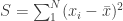
By inspection this is inverse gamma with parameters N/2, S/2, where S=\sum{(x_i-\mu)^2}.

So \sigma^2|\vec{x},\mu \sim  \mbox{invgamma}(N/2,S/2)

Note that we went from N-1 dof in the marginal-conditional sampling earlier to N dof in Gibbs sampling. This is because we already know \mu when sampling on \sigma^2|\vec{x},\mu but we did not know it when doing the marginal-conditional sampling. In the previous case the difference involves \bar{y}, but here it involves \mu.

We looked at a program to do this. Looked at some nice plots.

Started with \sigma^2=1000 (way off). What happens? The sampler very quickly moved to the region of interest.

But we wouldn’t want to include the first values in the posterior sample…they are anomalies. So often we run for a long time and discard some portion of the first samples. This is the “burn-in”.

Showed trace plot for \mu and \sigma for this example (starting way off). The ones he showed illustrated good mixing.

Convergence issues are the “Achilles’ heel” of MCMC. There are no accepted standards for convergence. You have to be very careful, because you may not have sampled the whole sample space. Sampling from various starting points. Winbugs code to start from multiple places to see if you get the same results. What’s really problematic are multimodal posterior distributions. There are methods to handle these, but they are not trivial to implement.